
| Index A I | 機械学習Sample |
|
手書き文字 データ準備 分類器 学習 学習結果 予測 分類器変更 pkl保存 my_img推論 BostonHouse データ準備 WineQuality 構成・方式など タスク 導入 Sample 用語 |
sampleなどはCentOS7で実施 $ python3 $ python3 xxxx.py手書き文字 ・手書き文字の準備(学習データと教師データをロード) グレイスケールの手書き数字の画像データ1797個分をが行列形式で準備 データセットは8x8の画像が1797枚 それぞれに0〜9のラベルがついている。 images
    >>> from sklearn.datasets import load_digits    # 8x8の0から9の手書き文字
    >>> images = load_digits()
    >>> data = images.data    # 学習データ
    >>> target = images.target    # 教師データ(ラベル)
・トレーニング用とテスト用のデータを準備 全体のデータの2割を検証用に使用
    >>> from sklearn import model_selection
    >>> X_train, X_test, y_train, y_test =
     model_selection.train_test_split(data, target, test_size=0.2, random_state=0)
    >>> print(X_train.shape)    # フォーマット
     (1437, 64)
    >>> print(y_train.shape)
     (1437,)
    >>> print(X_test.shape)
     (360, 64)
    >>> print(y_test.shape)
     (360,)
    >>> print(X_train)    # データ
    [[ 0.  0.  0. ... 16. 16.  6.]
     [ 0.  3. 12. ... 16.  2.  0.]
     [ 0.  1. 10. ...  0.  0.  0.]
     ...
     [ 0.  0.  5. ...  0.  0.  0.]
     [ 0.  0.  4. ...  0.  0.  0.]
     [ 0.  0.  6. ... 11.  0.  0.]]
    >>> print(y_train)
    [6 5 3 ... 7 7 8]
    >>> print(len(y_test))    # データ数
    360
・判別器(分類器、識別器)にSVMを使用、X_train、y_trainで学習させて、X_testのラベルを予測 gammaとCの2個ののハイパーパラメータを指定 clf:classifier(分類器)
    >>> from sklearn import svm    # SVMインポート
    >>> clf = svm.SVC(gamma=0.001, C=100.)    # γ:大きいほど境界が複雑、C:誤分類の許容量
・学習 fit:fitted
>>> clf.fit(X_train,y_train)
・学習結果 (classifier.fit(train_X,train_y))
    SVC(C=100.0, break_ties=False, cache_size=200, class_weight=None, coef0=0.0,
        decision_function_shape='ovr', degree=3, gamma=0.001, kernel='rbf',
        max_iter=-1, probability=False, random_state=None, shrinking=True,
        tol=0.001, verbose=False)
・予測 pred:predicted(予測した) ラスト20のチェック
    >>> pred_test = clf.predict(X_test[-20:])     # 予測ラベル
    >>> print(pred_test)
    [5 1 6 4 5 0 9 4 1 1 7 0 8 9 0 5 4 3 8 8]
    >>> print(y_test[-20:])     # 正解ラベル
    [5 1 6 4 5 0 9 4 1 1 7 0 8 9 0 5 4 3 8 8]
全体
    >>> from sklearn.metrics import accuracy_score
    >>> pred_test = clf.predict(X_test)
    >>> accuracy_test = accuracy_score(y_test,pred_test)
    >>> print(accuracy_test)
    0.9916666666666667
・分類器を「svm.LinearSVC()」に
    >>> clf = svm.LinearSVC()
    >>> clf.fit(X_train,y_train)
    >>> pred_test = clf.predict(X_test)
    >>> accuracy_test = accuracy_score(y_test,pred_test)
    >>> print(accuracy_test)
    0.9361111111111111
・学習済みデータをPickle形式で保存
    >>> data = images.data
    >>> target = images.target
    >>> from sklearn import model_selection
    >>> X_train, X_test, y_train, y_test =
     model_selection.train_test_split(data, target, test_size=0.2, random_state=0)
    >>> from sklearn import svm
    >>> clf = svm.SVC(gamma=0.001, C=100.)
    >>> clf.fit(X_train,y_train)
    SVC(C=100.0, break_ties=False, cache_size=200, class_weight=None, coef0=0.0,
        decision_function_shape='ovr', degree=3, gamma=0.001, kernel='rbf',
        max_iter=-1, probability=False, random_state=None, shrinking=True,
        tol=0.001, verbose=False)
    >>> save_file = 'digits.pkl'    # 拡張子、pkl
    >>> with open(save_file, 'wb') as f:
    ...     pickle.dump(clf, save_file, f, -1)    # -1、最も高いプロトコルバージョンで保存
    ...     print(clf)
    ...
    SVC(C=100.0, break_ties=False, cache_size=200, class_weight=None, coef0=0.0,
        decision_function_shape='ovr', degree=3, gamma=0.001, kernel='rbf',
       max_iter=-1, probability=False, random_state=None, shrinking=True,
       tol=0.001, verbose=False)
    >>>
・自分で書いたmy_img(手書きの数字)文字をテスト
(推論) 「PIL、numpy」を使用、「skimage、io」でもよい xxxx.py #!/usr/bin/env python3 # from PIL import Image import numpy as np import pickle #my_img = np.array(Image.open('9.png')) my_img = np.array(Image.open('9.png').convert('L')) # 2次元で取り込み print("my_img =", type(my_img)) print("dtype =", my_img.dtype) print("shape =", my_img.shape) # 大きい場合はresize Image.fromarray(my_img).save('9_1.png')  #my_img = 15 - my_img // 16 my_img = my_img.reshape([-1,64]) file = open('digits.pkl', 'rb') Pickle形式で保存済 clf = pickle.load(file) res = clf.predict(my_img) print("my_img = " + str(res[0])) print("End") 実行結果
    my_img = <class 'numpy.ndarray'>
    dtype = uint8
    shape = (8, 8)
    my_img = 2
    End
・sklearn.metricsを使って検証
    >>> from sklearn.metrics import confusion_matrix
    >>> predicted = fitted.predict(X_test)
    >>> metrics.confusion_matrix(predicted, y_test)
    array([[27,  0,  0,  0,  0,  0,  0,  0,  0,  0],
           [ 0, 35,  0,  0,  0,  0,  0,  0,  0,  0],
           [ 0,  0, 36,  0,  0,  0,  0,  0,  0,  0],
           [ 0,  0,  0, 29,  0,  0,  0,  0,  0,  0],
           [ 0,  0,  0,  0, 30,  0,  0,  0,  0,  0],
           [ 0,  0,  0,  0,  0, 40,  0,  0,  0,  0],
           [ 0,  0,  0,  0,  0,  0, 44,  0,  0,  0],
           [ 0,  0,  0,  0,  0,  0,  0, 39,  0,  0],
           [ 0,  0,  0,  0,  0,  0,  0,  0, 39,  0],
           [ 0,  0,  0,  0,  0,  0,  0,  0,  0, 41]])
boston_house_prices ・$ python3 (重回帰分析)
    >>> import pandas as pd
    >>> import numpy as np
    >>> import matplotlib.pyplot as plt
    >>> from sklearn import datasets
    >>> from sklearn import linear_model
    >>> from sklearn import model_selection
    >>> from sklearn.preprocessing import StandardScaler
    >>> boston = datasets.load_boston()    # ロード
    >>> data = boston.data
    >>> target = boston.target
    >>> print(data.shape)
    (506, 13)
    >>> print(target.shape)
    (506,)
・トレーニング用とテスト用のデータを準備 全体のデータの2割をテスト証用、2割を検証用に
    >>> X_train, X_test, y_train, y_test =
     model_selection.train_test_split(data, target, test_size=0.2, random_state=114514)
    >>> print(X_train.shape)    # フォーマット
     (404, 13)
    >>> print(y_train.shape)
     (404,)
    >>> print(X_test.shape)
     (102, 13)
    >>> print(y_test.shape)
     (102,)
    >>> print(X_train)    # データ
    [[1.77800e-02 9.50000e+01 1.47000e+00 ... 1.70000e+01 3.84300e+02
      4.45000e+00]
     [2.29270e-01 0.00000e+00 6.91000e+00 ... 1.79000e+01 3.92740e+02
      1.88000e+01]
     [4.07710e-01 0.00000e+00 6.20000e+00 ... 1.74000e+01 3.95240e+02
      2.14600e+01]
     ...
     [4.22239e+00 0.00000e+00 1.81000e+01 ... 2.02000e+01 3.53040e+02
      1.46400e+01]
     [1.78667e+01 0.00000e+00 1.81000e+01 ... 2.02000e+01 3.93740e+02
      2.17800e+01]
     [3.75780e-01 0.00000e+00 1.05900e+01 ... 1.86000e+01 3.95240e+02
      2.39800e+01]]
    >>> print(y_train)
    [32.9 16.6 21.7 28.7 36.  22.6 16.7 16.  34.6 19.1 19.8 20.7 20.6 25.2
     27.1 50.  30.7 25.  18.7 26.5 27.9 23.9 17.5 23.1 22.  22.7 22.9 27.9
     50.  17.6 20.6 50.  45.4 17.5 35.2 20.1 21.8  6.3 18.8 20.9  9.6 21.4
     14.3 18.4 20.7 23.7 24.4 23.1 22.4 24.1 19.  18.4 20.4  7.  17.2 14.
     23.2 20.2 13.5 23.9 24.1 30.8 46.7 24.6 18.6 22.7 21.4 15.2 15.2 19.3
      8.1 24.3 34.9 14.4 23.1 23.6 28.7 26.4 13.1 13.9 23.1 50.  13.1 50.
     14.6 18.8 20.4 20.9 14.6 21.2 32.2 50.  26.2  5.  50.  13.9 23.1 12.6
     25.  10.8 21.  24.4 19.4 24.7 37.9 14.1 20.1 24.3 19.  19.1 19.4 11.8
     29.6 18.9 18.2 18.2 23.1 13.8 24.8 24.5 16.5 22.8 19.6 26.6 27.5 21.9
     20.8  5.  24.5 19.9  8.3 25.3 19.4 24.4 33.1  7.  24.8 31.5 15.  22.2
     13.1 22.6 34.9 17.1 21.  11.9 13.6  8.8 21.6 13.8 28.  15.  23.3 32.5
     21.4 30.1 23.7 41.3 18.  10.4 20.6 22.9 14.5 24.1 22.  50.  19.8 18.9
     29.6 32.  13.3 22.5 15.4 21.5 23.8 50.  13.5 22.  18.1 17.  50.  33.1
     21.7 18.2 10.2 22.2 24.5 34.7 33.2 23.  19.9 43.5 25.  23.6 42.8 16.3
     23.9 20.8 19.5 31.7 37.6 25.  19.7 16.1 14.2 21.2 17.1 36.2 20.3  8.7
     14.4  9.5 15.7 23.2 32.4 22.6 23.  48.3 50.  23.3 20.1 21.7 25.1 22.8
     33.  19.1 17.8 50.  16.1 15.6 14.9 15.6 17.5 27.5 17.8 13.  21.7  9.7
     25.  25.  38.7 31.2 19.5 36.4 32.  28.4 22.6 18.7 48.8 15.1 12.5 21.7
     23.5 30.1 24.  35.4 33.8 18.3 12.1 35.4 23.3 14.1 28.2 15.4 20.3 28.1
     26.6 21.2 31.6 41.7 10.5 23.7 12.7 19.6 17.4 20.4 11.5 23.  20.5 16.5
     25.  11.9 22.2 15.3 22.9 17.2 44.  21.5 11.7 24.6 17.8 50.  19.8 37.3
     18.6 22.8 13.8 24.  21.4 22.5 23.3 18.3  8.4 29.  12.7 15.6 19.1 20.
     19.4 29.  23.9 23.8 20.6 42.3 27.5 19.2 16.8 23.4 21.7 20.1 22.2 16.1
     30.1 32.7 23.7 19.3 18.5 22.4 11.8 21.2 22.  22.2 14.9 20.2 14.5 22.1
     19.3 13.8 28.4 17.3 29.8 24.7 21.7 28.5 18.4 19.5 18.5 35.1 22.  20.8
     37.2 17.4 10.5 23.2 17.8 24.8 21.2 27.5 14.3 23.8 18.7 46.   8.8 22.5
     16.2 29.1 10.4 11.7 24.7  5.6 21.1 20.4 17.9 21.8 39.8 31.1 13.3 20.3
     14.1 22.3  8.3 13.2 13.4 18.5 43.1 27.  31.6 12.3 18.9 33.3  8.5 17.2
     22.  26.7 24.8 19.6 11.3 29.1 17.8 20.5 20.5 16.8 10.2 19.3]
・$ python3 (SGD)
>>> import pandas as pd
>>> import numpy as np
>>> import matplotlib.pyplot as plt
>>> from sklearn import datasets
>>> from sklearn import linear_model
>>> from sklearn.preprocessing import StandardScaler
>>> from sklearn.preprocessing import MinMaxScaler
>>> boston = datasets.load_boston() # ロード
>>> print(boston)
>>> print(boston.DESCR)
>>> print(boston.data)
>>> print(boston.feature_names)
>>> print(boston.target)
>>> boston_df=pd.DataFrame(boston.data) # DataFrameセット
>>> boston_df.columns = boston.feature_names
>>> boston_df['PRICE'] = pd.DataFrame(boston.target)
>>> boston_df.to_csv('boston_df.csv', sep=',', index=True, encoding='utf-8') # csv出力
>>> boston_df.to_csv('boston.csv', sep=',', index=False, encoding='utf-8')
>>> X = boston_df.drop("PRICE", axis=1) # Xセット
>>> mscaler = MinMaxScaler()
>>> mscaler.fit(X) # Xを正規化(Normalization)
>>> X2 = mscaler.transform(X)
>>> X2 = pd.DataFrame(X2)
>>> X2.columns = boston.feature_names
>>> print("X2.describe() ->")
>>> print(X2.describe())
>>> Y = boston_df.PRICE # Yセット
>>> clf2_SGD = linear_model.SGDRegressor(max_iter=500) # SGDRegressorで分析
>>> clf2_SGD.fit(X2, Y) # 事前に正規化済
SGDRegressor(alpha=0.0001, average=False, early_stopping=False, epsilon=0.1,
eta0=0.01, fit_intercept=True, l1_ratio=0.15,
learning_rate='invscaling', loss='squared_loss', max_iter=500,
n_iter_no_change=5, penalty='l2', power_t=0.25, random_state=None,
shuffle=True, tol=0.001, validation_fraction=0.1, verbose=0,
warm_start=False)
>>> print("### out put from X2 data and used SGD ###############")
>>> print(pd.DataFrame({"Name":X2.columns,
"Coefficients":clf2_SGD.coef_}).sort_values(by='Coefficients') ) # 係数でソート
Name Coefficients
12 LSTAT -17.527713
10 PTRATIO -7.573122
7 DIS -7.196724
9 TAX -3.927853
0 CRIM -3.924537
4 NOX -3.311751
2 INDUS -0.303527
6 AGE 1.106992
1 ZN 2.933184
3 CHAS 3.072527
8 RAD 4.119741
11 B 5.686851
5 RM 23.888114
>>> print(clf2_SGD.intercept_) # 切片
[16.97465888]
>>> print(clf2_SGD.score(X2,Y)) # R^2
0.7250366947774292
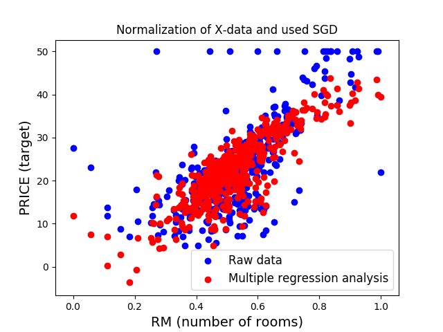
# plot output
>>> plt.figure(1)
>>> plt.title('Normalization of X-data and used SGD')
>>> plt.xlabel('RM (number of rooms)', fontsize=14)
>>> plt.ylabel('PRICE (target)', fontsize=14)
>>> plt.scatter(X2.RM, Y, c='blue', label='Raw data')
>>> plt.scatter(X2.RM, clf2_SGD.predict(X2), c='red', label='Multiple regression analysis')
>>> plt.legend(loc='lower right', fontsize=12)
>>> #plt.show()
>>> plt.savefig("exampleClf2_SGD.png")
 Wine Quality Data Set ・$ python3 winequality-red.py
    #!/usr/bin/env python3
    #
    import pandas as pd
    import numpy as np
    import matplotlib.pyplot as plt
    from sklearn.linear_model import LinearRegression

    pd.set_option("display.max.columns", 100)
    pd.set_option("display.max.rows", 100)

    wine = pd.read_csv("winequality-red.csv",sep=";")

    print("wine.shape->")
    print(wine.shape)
    print("wine.head->")
    print(wine.head())
    print("wine.tail->")
    print(wine.tail())

    wine_eccept_quality = wine.drop("quality", axis=1)
    X = wine_eccept_quality.values
    Y = wine['quality'].values

    clf = LinearRegression(fit_intercept=True, normalize=False, copy_X=True, n_jobs=1)
    clf.fit(X,Y)

    print("pd.DataFrame->")
    print(pd.DataFrame({"Name":wine_eccept_quality.columns, "Coefficients":clf.coef_})
    .sort_values(by='Coefficients') )
    #print("clf.coef_->", clf.coef_)
    print("clf.intercept_->", clf.intercept_)
    print("clf.score->", clf.score(X,Y))
    print("End")
・winequality-red.py実行結果
    wine.shape->
    (1599, 12)
    wine.head->
       fixed acidity  volatile acidity  citric acid  residual sugar  chlorides  \
    0            7.4              0.70         0.00             1.9      0.076
    1            7.8              0.88         0.00             2.6      0.098
    2            7.8              0.76         0.04             2.3      0.092
    3           11.2              0.28         0.56             1.9      0.075
    4            7.4              0.70         0.00             1.9      0.076

       free sulfur dioxide  total sulfur dioxide  density    pH  sulphates  \
    0                 11.0                  34.0   0.9978  3.51       0.56
    1                 25.0                  67.0   0.9968  3.20       0.68
    2                 15.0                  54.0   0.9970  3.26       0.65
    3                 17.0                  60.0   0.9980  3.16       0.58
    4                 11.0                  34.0   0.9978  3.51       0.56

       alcohol  quality
    0      9.4        5
    1      9.8        5
    2      9.8        5
    3      9.8        6
    4      9.4        5
    wine.tail->
          fixed acidity  volatile acidity  citric acid  residual sugar  chlorides  \
    1594            6.2             0.600         0.08             2.0      0.090
    1595            5.9             0.550         0.10             2.2      0.062
    1596            6.3             0.510         0.13             2.3      0.076
    1597            5.9             0.645         0.12             2.0      0.075
    1598            6.0             0.310         0.47             3.6      0.067

          free sulfur dioxide  total sulfur dioxide  density    pH  sulphates  \
    1594                 32.0                  44.0  0.99490  3.45       0.58
    1595                 39.0                  51.0  0.99512  3.52       0.76
    1596                 29.0                  40.0  0.99574  3.42       0.75
    1597                 32.0                  44.0  0.99547  3.57       0.71
    1598                 18.0                  42.0  0.99549  3.39       0.66

          alcohol  quality
    1594     10.5        5
    1595     11.2        6
    1596     11.0        6
    1597     10.2        5
    1598     11.0        6
    pd.DataFrame->
                        Name  Coefficients
    7                density    -17.881164
    4              chlorides     -1.874225
    1       volatile acidity     -1.083590
    8                     pH     -0.413653
    2            citric acid     -0.182564
    6   total sulfur dioxide     -0.003265
    5    free sulfur dioxide      0.004361
    3         residual sugar      0.016331
    0          fixed acidity      0.024991
    10               alcohol      0.276198
    9              sulphates      0.916334
    clf.intercept_-> 21.965208449451552
    clf.score-> 0.36055170303868855
    End
・ワインの品質スコアの回帰式
    [quality] = -17.881164 * [density] + -1.874225 * [chlorides] +
                -1.083590 * [volatile acidity] + -0.413653 * [pH] +
                -0.182564 * [citric acid] + 0.016331 * [residual sugar] +
                0.004361 * [free sulfur dioxide] + -1.874225 * [chlorides] +
                0.024991 * [fixed acidity] + 0.276198 * [alcohol] +
                0.916334 * [sulphates] + 21.965208449451552
・$ python3 winequality-red_Norm.py (各変数を正規化して重回帰分析)
    #!/usr/bin/env python3
    #
    import pandas as pd
    import numpy as np
    import matplotlib.pyplot as plt
    from sklearn.linear_model import LinearRegression
    from sklearn.preprocessing import MinMaxScaler

    pd.set_option("display.max.columns", 100)
    pd.set_option("display.max.rows", 100)

    wine = pd.read_csv("winequality-red.csv",sep=";")
    #print("wine->")
    #print(wine)

    wine2 = wine.apply(lambda x:(x - np.mean(x)) / (np.max(x) - np.min(x)))
    wine2.head()

    wine2_eccept_quality = wine2.drop("quality", axis=1)
    X = wine2_eccept_quality.values
    Y = wine2['quality'].values

    clf = LinearRegression(fit_intercept=True, normalize=True, copy_X=True, n_jobs=1)
    clf.fit(X,Y)

    print("pd.DataFrame->")
    print(pd.DataFrame({"Name":wine2_eccept_quality.columns,
     "Coefficients":np.abs(clf.coef_)}).sort_values(by='Coefficients') )
    print("clf.coef_->", clf.coef_)
    print("clf.intercept_->", clf.intercept_)
    print("clf.score->", clf.score(X,Y))
    print("End")
・winequality-red_Norm.py実行結果
    pd.DataFrame->
                        Name  Coefficients
    2            citric acid      0.036513
    3         residual sugar      0.047687
    7                density      0.048708
    0          fixed acidity      0.056479
    5    free sulfur dioxide      0.061931
    8                     pH      0.105068
    6   total sulfur dioxide      0.184775
    4              chlorides      0.224532
    9              sulphates      0.306056
    1       volatile acidity      0.316408
    10               alcohol      0.359057
    clf.coef_-> [ 0.05647865 -0.31640836 -0.03651279  0.04768731 -0.22453217  0.06193093
     -0.18477521 -0.04870829 -0.1050679   0.30605569  0.35905701]
    clf.intercept_-> 1.9140742913275685e-16
    clf.score-> 0.3605517030386882
    End
・ワインの品質への各変数の影響度を、偏回帰係数の大小で比較 「alcohol(アルコール度数)」が品質に大きな影響を与えている。 |
| All Rights Reserved. Copyright (C) ITCL | |